


I. Introduction
The dynamics of housing markets have become increasingly significant in economic research and policymaking due to their profound implications for financial stability, wealth distribution, and urban development in South Korea. Momentum effects, which refer to the persistence of past price trends influencing future prices, have been extensively documented in various asset markets, including equities (Jegadeesh & Titman, 1993). However, the presence and impact of momentum effects in housing markets remain an area of active investigation, particularly in East Asian economies like South Korea. Existing research on housing market dynamics has primarily focused on developed Western markets, particularly the United States (Case & Shiller, 1989; Piazzesi & Schneider, 2009), leaving a gap in understanding how momentum manifests in South Korea’s unique housing context. This study seeks to address this gap by investigating the factors that drive housing price movements in South Korea, including regional heterogeneity.
Understanding momentum effects in housing prices is crucial for policymakers and investors due to the far-reaching implications for market stability and wealth distribution. Previous studies, such as Piazzesi & Schneider (2009), have demonstrated the role of momentum traders in driving price cycles in the U.S. housing market, leading to price booms and busts. The risk associated with momentum effects is further exacerbated in markets with high household debt levels, as shown by Glaeser & Nathanson (2015), who emphasized how momentum traders can inflate housing bubbles with severe economic consequences when they burst. South Korea’s housing market, characterized by significant household debt tied to real estate, represents a critical environment for exploring these dynamics. South Korea’s household debt-to-GDP ratio has consistently been among the highest in the world, raising concerns about the potential impact of momentum-driven price cycles on household wealth and financial stability.
The presence of momentum effects in housing prices also raises important questions about the efficiency of real estate markets. According to the efficient market hypothesis (EMH), asset prices should fully reflect all available information, implying that future price movements are unpredictable and follow a random walk (Fama, 1970). However, the detection of momentum effects, where past price trends can predict future price movements, suggests a deviation from market efficiency. In housing markets, several studies have documented such inefficiencies. For instance, Case & Shiller (1989) found that U.S. housing markets exhibit mean-reverting behavior over the long term, suggesting that prices do not always reflect fundamental values. Similarly, Poterba (1991) provided evidence that U.S. cities often experience price trends that persist for several years before correcting, indicating a potential lag in the incorporation of new information. In the context of South Korea, our findings that some regions exhibit strong local momentum effects while others show tendencies toward mean reversion further challenge the assumption of market efficiency. These dynamics imply that local market conditions, transaction costs, and policy interventions may contribute to inefficiencies, creating opportunities for strategic investment but also heightening the risk of price bubbles and subsequent corrections. Thus, understanding the dynamics and triggers behind deviations of housing markets from EMH can offer valuable insights for policymakers and investors in navigating these complex market environments.
In South Korea, the study of momentum effects in housing prices is still emerging, with limited research exploring the regional differences in market behavior. Previous studies, such as the work by Choi (2024),1) have explored regional variations in housing markets but have largely focused on price indices rather than transaction-level data. Using monthly, transaction-level data, this study offers a more granular perspective on South Korea’s housing price dynamics—an approach largely absent from the existing literature. Unlike prior research that relies on aggregate price indices, this study captures market nuances, including the influence of transaction volume and price volatility on housing price momentum. Our findings provide new insights into the spatial and temporal variability of momentum effects. In particular, when combining the national-level average effect with city-level deviations, the overall momentum effect tends to be weak, suggesting a tendency toward mean reversion in housing prices. However, this aggregate pattern masks significant regional variation. In certain cities such as Seoul, local momentum effects are relatively strong and partially counteract the national mean-reverting trend, leading to more persistent—but not fully momentum-driven—price dynamics in those areas. This underscores the importance of accounting for spatial heterogeneity when analyzing housing market behavior, as regional deviations may meaningfully shape local market trajectories even when national trends point toward mean reversion.
In terms of methodology, this study employs various model specifications to explore the factors influencing housing price trends in Korea, ranging from simple baseline models to more comprehensive ones that consider regional effects and market activity-related information. Specifically, to capture regional heterogeneity, we implement a Bayesian multilevel hierarchical approach, allowing us to model the variations in momentum effects across cities and districts. This approach aligns with the recommendations of Fingleton (2008) and Meen (2001) on the necessity of accounting for spatial differences in housing markets. The Bayesian hierarchical model results indicate that city-level momentum effects vary substantially across different regions in South Korea, with Seoul displaying strong positive momentum, while cities like Daegu and Incheon exhibit tendencies toward price correction. District-level characteristics, such as proximity to central business districts and infrastructure development, also significantly impact momentum effects. These findings suggest that regional differences in market dynamics are a key driver of housing price movements in South Korea.
A novel contribution of this study is the simulation of momentum strategies under various investment horizons, incorporating real-world frictions such as taxes and transaction fees. While earlier studies on momentum strategies in housing markets (Clayton, 1997) and recent work on local market conditions (Gao et al., 2020) have offered valuable insights, they often overlook the impact of transaction costs and taxes. Our analysis provides a more realistic assessment of momentum-based investing in the Korean housing market by simulating strategies with different formation and holding periods. The simulation results reveal that the momentum strategy’s effectiveness is significantly constrained when accounting for market frictions. Negative returns are observed consistently across various combinations of formation and holding periods, with the most pronounced losses occurring in short formation and holding periods. This outcome suggests that frequent trading in the Korean housing market is not viable due to the high transaction costs and tax burdens that erode potential profits.
By filling a gap in the existing literature and providing a comprehensive analysis of momentum effects in the South Korean housing market, this study aims to offer valuable insights for policymakers, investors, and researchers seeking to understand the complexities of housing price dynamics and develop targeted policies to mitigate risks associated with market volatility and high household debt levels.
To achieve these objectives, the study is structured around the following research questions:
-
Do housing price changes in South Korea exhibit momentum or mean-reversion dynamics, and how do these effects vary across cities and districts?
-
What is the predictive performance of hierarchical models that incorporate city- and district-level heterogeneity in momentum effects?
-
Can momentum-based investment strategies in the Korean housing market deliver positive returns once real-world frictions (e.g., taxes, fees, no short-selling) are accounted for?
These questions are addressed through the formulation of the following testable hypotheses:
-
- H1: Housing price changes in South Korea exhibit significant regional variation in momentum dynamics, with some areas showing local persistence and others mean reversion.
-
- H2: A hierarchical Bayesian model incorporating city- and district-level random effects provides superior predictive accuracy over simpler models.
-
- H3: Momentum-based trading strategies fail to produce excess returns under realistic tax and transaction cost constraints.
The remainder of this paper is structured as follows: Section 2 outlines the methodology, including the hierarchical models and identification strategy used to capture city- and district-level effects. Section 3 describes the data, emphasizing the use of monthly transaction-level information and the inclusion of various control variables. Section 4 presents the empirical results, examining the impact of city- and district-level characteristics on housing price momentum. Section 5 discusses the simulation of momentum strategies under different market conditions, highlighting the influence of taxes and fees on strategy performance. Finally, Section 6 concludes with a discussion of the study’s policy implications, limitations, and potential avenues for future research.
II. Methodology
In this study, we employ a Bayesian hierarchical model to investigate price momentum in South Korea’s apartment market while accounting for regional heterogeneity at the city and district levels. This approach is motivated by the need to capture the variation in how different local housing markets respond to recent price changes, which may be influenced by diverse economic conditions, regulatory environments, and market liquidity. By incorporating random slopes across spatial levels, our model builds on the tradition of multilevel modeling in housing economics and provides a more granular perspective on local momentum patterns.
The core econometric model is defined as follows:
Where:
-
- Yijkt denotes the monthly rate of change in the price of apartment unit i, located in district k of city j, during month t. Price changes are computed as log differences of transaction prices per exclusive area between months: Yijkt = log(Pijkt) − log(Pijkt − 1) where Pijkt denotes transaction price per unit of exclusive area.
-
- Yijkt − 1 is the one-month lagged value of the housing price change, which serves as the core momentum variable. A positive coefficient on this term indicates persistence in price dynamics—i.e., that an increase (or decrease) in price last month tends to be followed by another increase (or decrease) this month. In particular, if the coefficient on Yijkt − 1 approaches 1, it suggests a high degree of persistence, meaning that past price changes almost fully carry over into the current period. Conversely, a coefficient close to zero implies little or no temporal dependence.
-
- β0 is the model intercept representing the average monthly rate of housing price change across all units and regions.
-
- β1 captures the national average momentum effect, i.e., the degree to which past price changes predict current ones on average. It can be also interpreted as the approximate percentage point change in the current month’s rate of price change associated with a 1% change in the previous month’s rate of change (i.e., the approximate national-level elasticity with respect to the previous month’s housing price change rate).
-
- αj and δk denote city-level and district-level momentum effects, respectively, which modify the local responsiveness to lagged price changes (i.e., approximate elasticity at the city-level and the district-level, respectively, in response to past month’s housing price change rate). These capture unobserved regional heterogeneity in the persistence of price movements.
-
- Xit measures the number of transactions involving unit i during month t. This serves as a proxy for market liquidity in that specific building or complex.
-
- Zit captures the price volatility for unit i in month t, measured as the SD of transaction prices across all sales of unit i during that month.
-
- єijkt is an idiosyncratic error term assumed to follow an i.i.d. normal distribution: єijkt ~ N(0,σ2).
All variables are aligned on a monthly basis, and the time index t corresponds to calendar months between January 2010 and December 2023. Lagged values (i.e., Yijkt−1) are constructed by linking transactions of the same apartment unit in consecutive months. This dynamic structure enables us to isolate and estimate the persistence of price trends across different local markets.
A key innovation of our model lies in its hierarchical structure. We allow the momentum coefficient to vary by city and district via the following random effects:
Where and are hyperparameters capturing the variability of momentum across cities and districts, respectively. The inclusion of both αj and δk allows the model to flexibly account for spatial heterogeneity in housing market behavior, consistent with the literature on local housing market segmentation (Fingleton, 2008; Gyourko & Tracy, 1991).
All unknown parameters are estimated using Bayesian methods, with the following prior distributions:
-
- Regression coefficients β0 through β3 are assigned diffuse normal priors: N(0, 102), allowing for a wide range of plausible values without imposing strong prior beliefs.
-
- The city-level and district-level momentum effects are modeled as:
Which allows for flexible deviations from the global average momentum, while maintaining a centered structure.
Which facilitate regularization with heavy tails, allowing for flexibility in modeling variance components and accommodating uncertainty, as recommended in hierarchical Bayesian modeling (Gelman, 2006).
These prior choices strike a balance between flexibility and stability, ensuring that parameter estimates remain well-behaved in the presence of noisy or sparse data at the regional level.2) This hierarchical modeling framework builds on prior empirical research on housing price dynamics by enabling region-specific momentum effects to be estimated in a statistically coherent manner (Case & Shiller, 1989; Fingleton, 2008; Meen, 2001). By integrating unit-level variables and spatially structured random effects, the model provides a comprehensive representation of localized momentum behavior in the Korean apartment market.
To estimate the model, we employ Markov chain Monte Carlo (MCMC) methods, which allow for the estimation of posterior distributions for all model parameters based on the observed transaction-level data. Convergence of the sampling process is assessed using standard Bayesian diagnostics, including potential scale reduction factors (R^) and effective sample sizes, to ensure the reliability of posterior inference.
III. Data
This study utilizes apartment transaction data from seven major metropolitan areas in South Korea: Seoul, Busan, Daegu, Incheon, Gwangju, Daejeon, and Ulsan. The data are sourced through the Open API provided by the Korea Real Estate Board and cover the period from January 2010 to December 2023. Each transaction record contains detailed information, including the transaction date, actual transaction price, construction year, exclusive area (in square meters), street name, and administrative location codes (i.e., city and district).
These transaction-level data offer a high-resolution view of housing market activity, enabling monthly tracking of price changes, liquidity conditions, and local heterogeneity. The inclusion of geographical identifiers allows for precise spatial aggregation, while timestamped pricing data supports the construction of dynamic price series at the apartment-unit level. This structure is well suited for identifying both aggregate trends and localized momentum effects across the South Korean housing market.
To ensure consistency in unit-level price tracking, we define a homogeneous housing unit as a group of transactions sharing the same fixed structural and locational attributes. Specifically, we construct a composite identifier based on the apartment complex name, street name, exclusive area (in square meters), construction year,3) and administrative district code (gu). This combination allows us to approximate unit-level consistency in the absence of a true unit ID in the raw data.4) This classification strategy enables us to compare price movements for units with stable physical and locational characteristics over time.5)
A unit is considered a repeatedly transacted apartment if it appears in the dataset with at least two distinct transaction records across different months during the 2010–2023 period. This repeat-sales structure is fundamental to capturing within-unit price dynamics and controlling for unobserved heterogeneity. After filtering and grouping, we identify a total of 31,998 unique apartment units that meet this repeated transaction criterion.
All analyses are conducted on a monthly frequency.6) For each apartment unit, we retain the last transaction observed within each calendar month. This sampling rule is designed to capture the most up-to-date market signal for each unit in each period, while avoiding distortions that may arise from averaging across heterogeneous or sparsely distributed transactions within the same month.7)
Months without any transaction for a given unit are treated as missing. We do not impute values for such months—either through last-observation-carried-forward (LOCF) or other imputation methods—because doing so may introduce artificial persistence or smoothness that does not reflect actual market activity. Furthermore, imputation methods inherently rely on assumptions that could introduce additional biases, particularly from the choice of the modeling approach. While this strategy leads to some degree of temporal sparsity, it helps preserve the integrity of the observed transaction process by clearly distinguishing between active and inactive periods, without artificially inflating market activity.
To account for market liquidity and price uncertainty, we construct two time-varying control variables at the unit level: (1) the number of transactions per unit-month and (2) price volatility within the unit-month.
-
- Transaction volume: For each unit and calendar month, we compute the total number of recorded transactions. This serves as a measure of liquidity or market activity surrounding the unit. Formally, for unit i in month t, transaction volume is defined as:
Where nit is the number of distinct transactions recorded for unit i during month t. While most units transact infrequently, instances of multiple trades within a single month do occur and are captured by this measure. A higher value of Xit reflects more active turnover or stronger demand in the submarket.
-
- Price volatility: For each apartment unit and month, we calculate the SD of transaction prices when two or more sales are recorded within that month. For unit i in month t, the price volatility is defined as:
Where Pijt denotes the j-th transaction price of unit i in month t, P̅it is the average price for that unit in that month, and nit is the number of transactions. If nit < 2, the volatility measure σit is set to missing. This conservative rule ensures that the volatility reflects genuine within-period price dispersion rather than noise from sparse observations.
Together, these covariates serve as critical controls in our empirical model. Transaction volume captures local market liquidity and trading intensity, while price volatility reflects the level of uncertainty or dispersion in price signals.
<Table 1> presents the summary statistics of the key variables used in the analysis. The average monthly return in apartment prices is approximately 0.65%, with a relatively high SD of 10.6 percentage points, indicating considerable variation in short-term price movements across units. Trading volume, measured as the log-transformed number of monthly transactions, exhibits right-skewed distribution with a median of 1.39 and a maximum of 5.71, suggesting that while most properties trade infrequently, a small subset experiences much higher turnover. Price volatility, defined as the log-transformed SD of within-month transaction prices, has a mean of 7.74 and ranges from 0 to over 13, reflecting substantial heterogeneity in price dispersion across units and time.
IV. Results
We used four different model specifications to study how previous price changes, city and district-specific factors, and other control variables affect housing prices. Below are the results from each model, highlighting important parameters like the effect of the national-level momentum effect (β1), city and district-level influences.
The baseline model, which only includes lagged home price changes (β1), gives us an understanding of the momentum effects in the South Korean housing market. <Table 2> summarizes the posterior distribution of the model parameters. The posterior mean of β1 is estimated at –0.437, with a narrow 90% highest density interval (HDI) ranging from –0.440 to –0.435. The small Monte Carlo standard errors (MCSE) and the R-hat value of 1 indicate convergence and reliability of the estimates.
Note: This table reports the posterior summaries for the baseline specification (Model 1). The posterior mean and SD represent the central tendency and dispersion of the estimated parameters. The 5% and 95% highest density intervals (HDIs) define the central 90% credible region for each parameter. Monte Carlo standard errors (MCSE) assess the numerical accuracy of the posterior mean and SD estimates. R-hat values close to 1 indicate satisfactory convergence across Markov chain Monte Carlo (MCMC) chains.
The negative estimate of β1 indicates that, under the baseline specification, housing prices tend to exhibit mean-reverting behavior rather than momentum. Specifically, the posterior mean of –0.437 implies that, holding other factors constant, an increase in the previous month’s price change is, on average, associated with a decline in the current month’s price change. This finding contrasts with the typical expectation of momentum effects, where past price changes lead to further increases in the following period. Instead, the results imply that periods of rapid price appreciation are likely followed by corrections.
This result aligns with previous studies on mean reversion in asset prices but differs in its timing. For example, Case & Shiller (1989) found mean-reverting behavior in the U.S. housing market, where periods of rapid price growth were followed by declines over the long term, driven by market corrections and economic adjustments. In contrast, our findings indicate that mean reversion occurs in the short run in the South Korean housing market. Similarly, Clayton (1997) suggested that while housing markets might exhibit short-term momentum, long-term price movements often revert to fundamental values. The negative lagged price change effect in our model suggests that the rapid appreciation of home prices in South Korea may prompt immediate corrective phases, highlighting a distinctive market dynamic compared to longer-term adjustments observed in other markets.
Although parsimonious, the baseline model accounts for a substantial share of the variation in housing price changes through the inclusion of the lagged price change variable. However, it leaves unexplained heterogeneity across different cities and districts. The posterior estimate for the residual SD (σ) is 0.106, indicating that the baseline specification captures some but not all of the dynamics in home price changes. This suggests that factors beyond past price changes, such as city-level and district-level heterogeneity, may play an important role in shaping housing price trajectories in South Korea.
In the following subsections, we extend this baseline model to incorporate spatial effects, such as city and district fixed effects, to better account for the observed heterogeneity across regions.
Model 2 extends the baseline specification by introducing city-level response parameters (αj), which capture the heterogeneity in how housing prices in each city react to lagged price changes. This allows for a more granular analysis of how different urban areas in South Korea experience momentum or mean-reversion effects in their housing markets. Summary statistics of the posterior distributions from Model 2 are presented in <Table 3>.
Note: This table reports the posterior summaries for the Model 2. The posterior mean and SD represent the central tendency and dispersion of the estimated parameters. The 5% and 95% highest density intervals (HDIs) define the central 90% credible region for each parameter. Monte Carlo standard errors (MCSE) assess the numerical accuracy of the posterior mean and SD estimates. R-hat values close to 1 indicate satisfactory convergence across Markov chain Monte Carlo (MCMC) chains. The parameter α[city] denotes the city-level momentum effect.
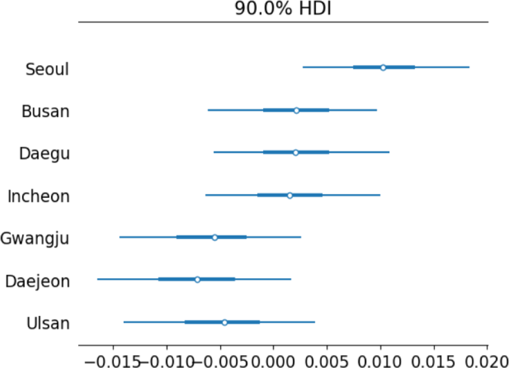
The posterior distribution for the national-level momentum effect (β1) indicates a significant negative relationship between past and current housing price changes. The mean estimate of β1 is –0.44, with a 90% HDI ranging from –0.446 to –0.433, reinforcing the evidence for mean reversion. However, we found that the city-level responses, captured by the αj parameters, show considerable variation across cities: Seoul exhibits a positive city-level effect, with a posterior mean of 0.011, suggesting that price changes in Seoul are more likely to partially offset the national mean-reverting trend and exhibit localized momentum, potentially driven by sustained demand and structural factors such as housing shortages and limited space for new home development projects. Busan, Daegu, and Incheon exhibit modest positive city-level effects, with posterior means approximately 0.002, indicating mild local momentum that partially counteracts the broader national mean-reverting trend. In contrast, Gwangju, Daejeon, and Ulsan exhibit negative city-level effects, with posterior means ranging from –0.005 to –0.007, indicating that price increases in these regions are more likely to be followed by subsequent declines—suggesting localized mean reversion, market corrections, or relatively weaker demand conditions.
<Fig. 1> presents the 90% HDIs for the city-level responses to lagged housing price changes. These intervals represent the uncertainty around the posterior estimates of the city-specific parameters in the model. The observed heterogeneity in city-level responses (αj) also highlights the importance of local factors in housing market dynamics. For example, the stronger positive response observed in Seoul suggests that its housing market is characterized by conditions conducive to sustained price appreciation, such as strong economic fundamentals, high population density, and constrained housing supply. On the other hand, cities like Gwangju and Daejeon may be more susceptible to corrections following price surges, reflecting weaker demand or a more elastic housing supply. This finding is consistent with the work of Meen (2001), who emphasizes the role of regional economic conditions and supply constraints in shaping housing price dynamics.
The findings from Model 2 indicate that housing markets in South Korea do not all show the same momentum effects. Instead, differences in local economic conditions, market-specific characteristics, and regulatory environments contribute to varying price dynamics across cities. This discovery has significant policy implications, suggesting that efforts to stabilize housing prices may need to be customized to the specific conditions of each city, rather than using a one-size-fits-all approach. The varying values of αj across cities indicate the need for a housing policy framework that takes into account local supply-demand imbalances, economic growth patterns, and housing market conditions.
Model 3 extends the analysis by simultaneously incorporating both city-level momentum effects (αj) and district-level effects (δk) nested within each city. This specification allows for a more nuanced understanding of housing price dynamics, recognizing that regional heterogeneity exists not only between cities but also within them. By modeling the effects at both the city and district levels, we account for the possibility that housing price behavior differs significantly within a city based on local neighborhood characteristics, infrastructure, and economic conditions.
While city-level effects capture broader economic, demographic, and policy factors that influence housing markets, district-level effects allow us to capture more localized variations that are often masked when only city-level dynamics are considered. For instance, within large metropolitan areas like Seoul, districts may vary widely in terms of housing supply constraints, socio-economic composition, and development potential. Ignoring these district-level variations could lead to an oversimplification of the housing price dynamics and misguide policy recommendations.8)
The results presented in <Table 4> demonstrate that the inclusion of district-level effects does not significantly alter the overall momentum effects at the city level, but it refines our understanding of how prices evolve within cities. The posterior mean for β1 remains consistent with previous models, estimated at –0.439 with a 90% HDI ranging from –0.446 to –0.432. This persistent negative relationship between lagged price changes and current price changes continues to suggest mean reversion.
Note: This table reports the posterior summaries for the Model 3. The posterior mean and SD represent the central tendency and dispersion of the estimated parameters. The 5% and 95% highest density intervals (HDIs) define the central 90% credible region for each parameter. Monte Carlo standard errors (MCSE) assess the numerical accuracy of the posterior mean and SD estimates. R-hat values close to 1 indicate satisfactory convergence across Markov chain Monte Carlo (MCMC) chains. The parameter α[city] denotes the city-level momentum effect. District-level momentum effects (δk) are not reported here due to the limited space.
However, the city-specific parameters (αj) reveal varied responses, as seen in the previous model. For example, Seoul exhibits a positive local momentum effect (mean estimate: 0.008), suggesting that lagged price changes in Seoul are more likely to drive further increases. In contrast, cities like Daejeon and Ulsan show negative momentum effects, with posterior means of –0.005, indicating a tendency toward mean reversion at the city level.
The consistency of these results across various model specifications increases confidence in the core findings. It demonstrates that the introduction of district-level effects in Model 3 does not substantially change the main estimates for city-level momentum effects. The posterior distribution of the residual SD (σ) remains steady at 0.106, indicating that the model fit aligns with previous specifications.
Furthermore, the additional variance parameters, such as the SD of city-level momentum effects (σα) and district-level effects (σδ), indicate the importance of accounting for both levels of heterogeneity. The estimates for σα (0.008) and σδ (0.012) suggest that while city-level effects capture significant variation in housing price behavior, district-level effects also play a crucial role in explaining local price dynamics. Ignoring these nested structures would overlook key aspects of within-city variation.
The results from Model 3 underscore the importance of formulating housing market policies that account for both city-level economic conditions and intra-city heterogeneity at the district-level. Interventions that target only aggregate city-wide indicators may be insufficient to address the diverse patterns of demand-supply imbalances and price dynamics observed across districts. The findings highlight the need for more granular, location-specific policy measures—particularly in metropolitan areas such as Seoul and Busan, where substantial variation exists across districts in terms of housing market behavior.
These findings add to the increasing body of literature that stresses the significance of multi-level modeling in housing markets. Previous studies have mainly focused on macro-level city or regional effects, or have overlooked the nested structure of city and district dynamics. By explicitly considering district-level effects, this study aligns with more recent literature that supports a more detailed approach to housing price analysis, as suggested by Fingleton (2008).
The figures below illustrate the estimated district-level momentum effects (δk) in various districts of major South Korean cities. These momentum effects represent the district-level responses to previous changes in housing prices, offering insights into the different dynamics within each urban area. The colors in the figures indicate the strength and direction of the momentum effect, with darker shades showing stronger negative effects and lighter shades (or yellow) representing stronger positive effects.
<Fig. 2(a)> displays the momentum effects across Seoul’s districts. The results reveal significant variation within the city, with certain districts like Dongdaemun-gu and Jungnang-gu showing strong local positive momentum (posterior mean: 0.0104 and 0.0119, respectively). On the other hand, Mapo-gu and Jongno-gu exhibit negative local momentum effects (posterior mean: –0.0089 and –0.0066, respectively). This variation between districts might reflect the diverse economic conditions, demand pressures, and housing market regulations across Seoul’s urban areas.
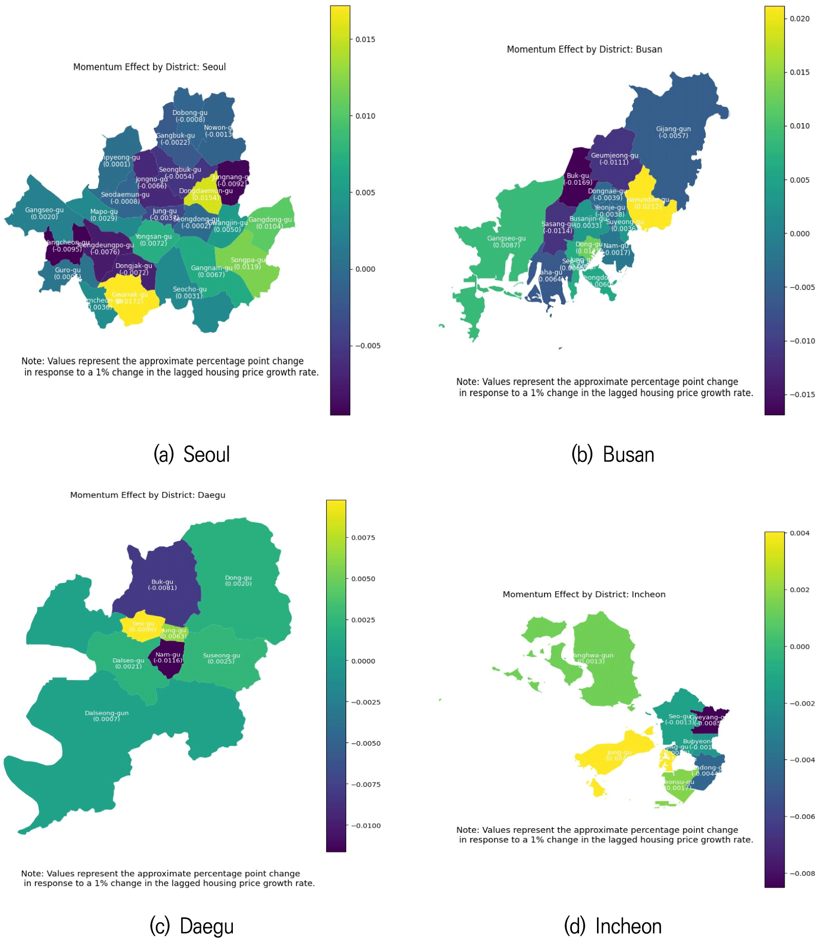
The Busan map (<Fig. 2(b)>) illustrates a similar heterogeneity in momentum effects across districts. Haeundae-gu shows the strongest positive local momentum with a posterior mean of 0.0212, likely driven by the district’s high desirability. Conversely, districts such as Buk-gu and Geumjeong-gu exhibit negative local momentum effects (posterior means: –0.0169 and –0.0111, respectively), indicating that these areas are more prone to price corrections after periods of price appreciation.
In Daegu (<Fig. 2(c)>), the spatial heterogeneity in housing momentum effects is also evident. Seo-gu and Jung-gu exhibit relatively strong positive local momentum effects, with posterior means of 0.0098 and 0.0063, respectively, indicating a pronounced tendency to counteract the national mean-reverting trend. On the other hand, Nam-gu displays a notable negative local momentum effect (–0.0116), signaling a higher likelihood of price reversals in this district.
<Fig. 2(d)> presents the momentum effects for Incheon. Districts such as Jung-gu and Namdong-gu demonstrate positive local momentum effects (posterior means: 0.0010 and 0.0017). In contrast, Seo-gu and Gyeyang-gu show negative local momentum effects (posterior means: -0.0013 and -0.0016), suggesting a reversion in prices after periods of appreciation. The district-level momentum effects in Gwangju (<Fig. 3(a)>) reveal that Dong-gu and Nam-gu have positive local momentum (posterior means: 0.0047 and 0.0043). On the other hand, Buk-gu and Seo-gu exhibit negative local momentum effects (–0.0096 and –0.0060), suggesting that housing markets in these areas are more prone to price corrections.
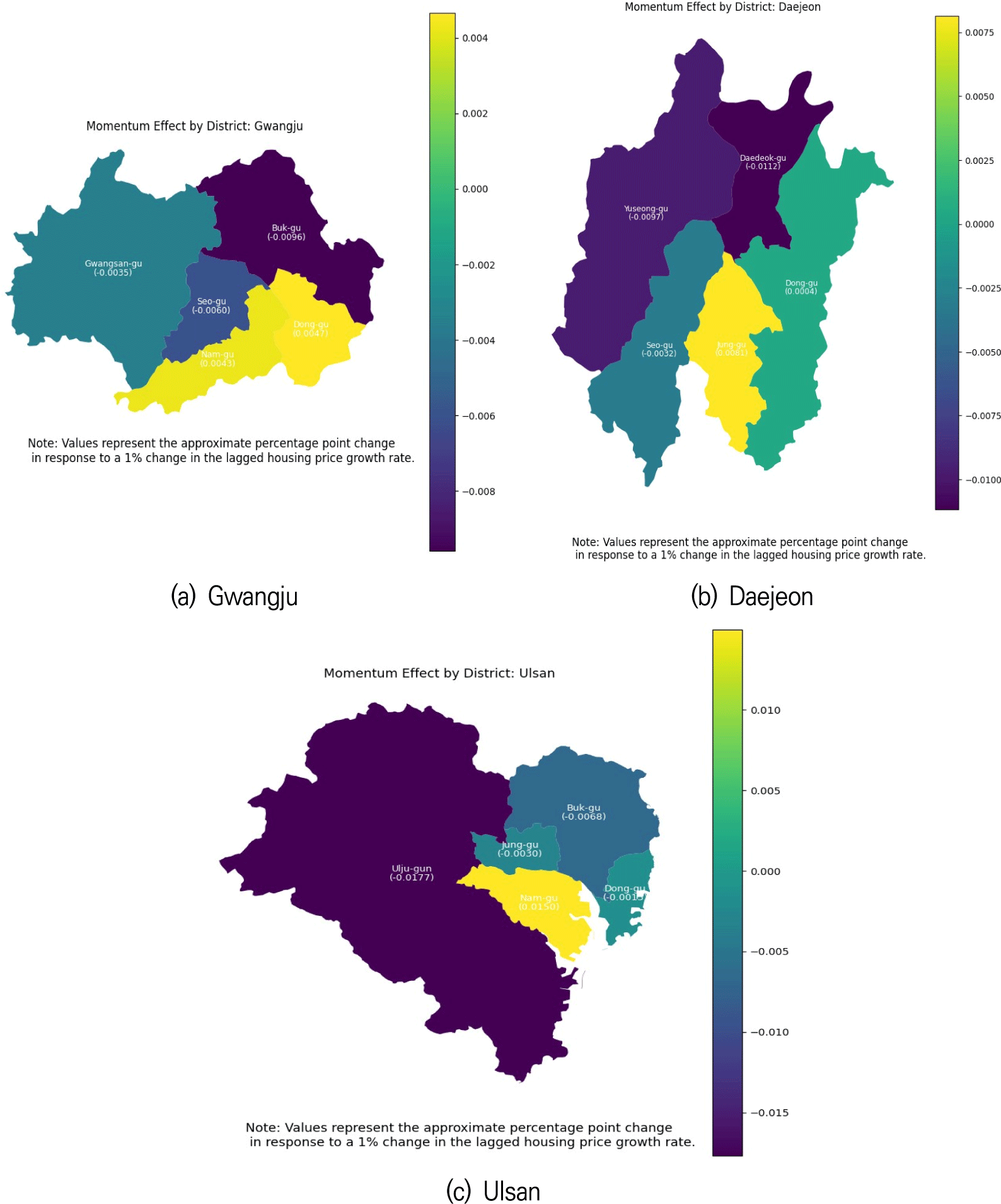
In Daejeon (<Fig. 3(b)>), Jung-gu shows the strongest positive local momentum effect, with a posterior mean of 0.0081. In contrast, Daedeok-gu and Yuseong-gu show significant negative local momentum (posterior means: –0.0112 and –0.0097). Finally, in Ulsan (<Fig. 3(c)>), Nam-gu exhibits a positive local momentum effect (posterior mean: 0.0035), while Buk-gu and Dong-gu show negative local effects (posterior means: –0.0092 and –0.0077). These results suggest that some districts in Ulsan may experience price reversion, likely influenced by industrial fluctuations and local economic factors that are unique to the city’s heavily industrialized environment.
Model 4 builds on the previous specifications by incorporating additional unit-level characteristics, specifically transaction volume and price volatility, alongside the existing city- and district-level momentum effects. These added covariates allow us to capture more granular dynamics that influence housing prices at a unit level. Transaction volume and price volatility provide valuable information about market liquidity and uncertainty, both of which are crucial determinants of price movements in housing markets. Including these variables helps improve the explanatory power of the model by accounting for short-term market fluctuations.9)
The results of Model 4, summarized in <Table 5>, show that the inclusion of transaction volume and price volatility does not significantly alter the core findings regarding city- and district-level momentum effects. The posterior mean for the national-level momentum effect (β1) remains strongly negative at –0.441, reaffirming the mean reversion effect observed in previous models.
Note: This table reports the posterior summaries for the Model 4. The posterior mean and SD represent the central tendency and dispersion of the estimated parameters. The 5% and 95% highest density intervals (HDIs) define the central 90% credible region for each parameter. Monte Carlo standard errors (MCSE) assess the numerical accuracy of the posterior mean and SD estimates. R-hat values close to 1 indicate satisfactory convergence across Markov chain Monte Carlo (MCMC) chains. The parameter α[city] denotes the city-level momentum effect. District-level momentum effects (δk) are not reported here due to the limited space.
The added variables provide additional insights into short-term market dynamics: (1) The transaction volume coefficient (β2) is positive with a mean estimate of 0.005 (90% HDI: 0.004, 0.005), indicating that higher transaction volumes are associated with increased housing prices. This result aligns with findings by Genesove & Mayer (2001), who showed that periods of high liquidity are often correlated with rising prices due to increased demand and market activity. (2) The price volatility coefficient (β3) is also positive, with a mean estimate of 0.002, suggesting that higher price volatility is associated with price increases. This finding is in line with the argument that volatility creates uncertainty, which can drive speculative behavior, leading to more rapid price changes (Engle et al., 1987).
At the city level, the momentum effects (αj) continue to exhibit heterogeneity across cities. Seoul exhibits a positive momentum effect, with a posterior mean of 0.008, suggesting that price increases in the city are more likely to persist over time, thereby counteracting the broader national tendency toward mean reversion. Conversely, cities such as Daejeon and Ulsan display negative momentum effects (posterior means: –0.007 and –0.005, respectively), suggesting a higher likelihood of price corrections following initial price increases.
One of the key strengths of Model 4 is that the inclusion of additional unit-level characteristics does not undermine the robustness of the core momentum effects observed at both the city and district levels. The national-level momentum effect remains consistently negative across all specifications, supporting the argument for mean reversion in housing prices. The inclusion of transaction volume and price volatility enriches the model by accounting for short-term liquidity and risk factors that drive housing market fluctuations.
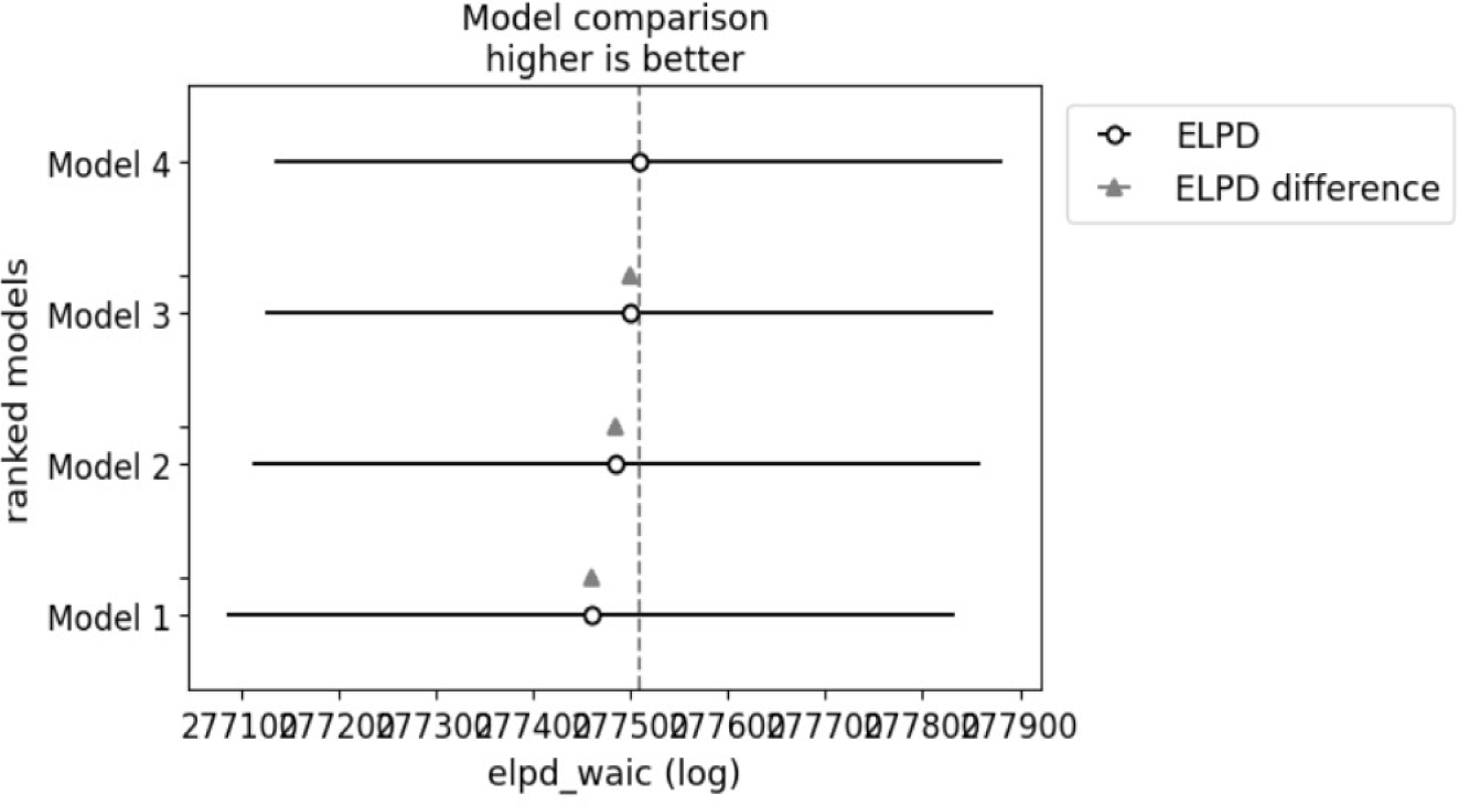
The empirical advantages of this extended specification are further supported by model comparison results. <Fig. 4> shows the WAIC-based model comparison across four competing specifications. Model 4, which includes city- and district-level random effects along with unit-level controls, achieves the highest ELPD value, indicating the best out-of-sample predictive performance. Models 3 and 2 show modest declines in fit, while Model 1 performs the worst. The clear separation in ELPD values suggests that incorporating multi-level structure and housing-specific covariates improves the model’s ability to capture systematic momentum patterns in housing prices.
To further investigate regional heterogeneity in housing price dynamics, we report the combined city-specific momentum coefficients (β1+αj) from Model 4 across seven major metropolitan housing markets. These composite estimates capture the responsiveness of the current month’s rate of price change to that of the previous month—interpreted as the approximate percentage point change in the current rate of price growth associated with a 1% change in the prior month. This formulation enables the identification of region-specific patterns of momentum or mean reversion in housing market behavior.
<Fig. 5> displays the posterior densities of the composite term, β1+αj, where β1 is the national-level momentum effect and αj captures city-specific effect. In our results, all cities show negative posterior means, suggesting that mean reversion dominates overall. Seoul exhibits the weakest mean reversion (closest to zero), while Daejeon and Ulsan exhibit the strongest reversion effects. These variations indicate spatially distinct housing market behaviors that are not captured by aggregate national models.
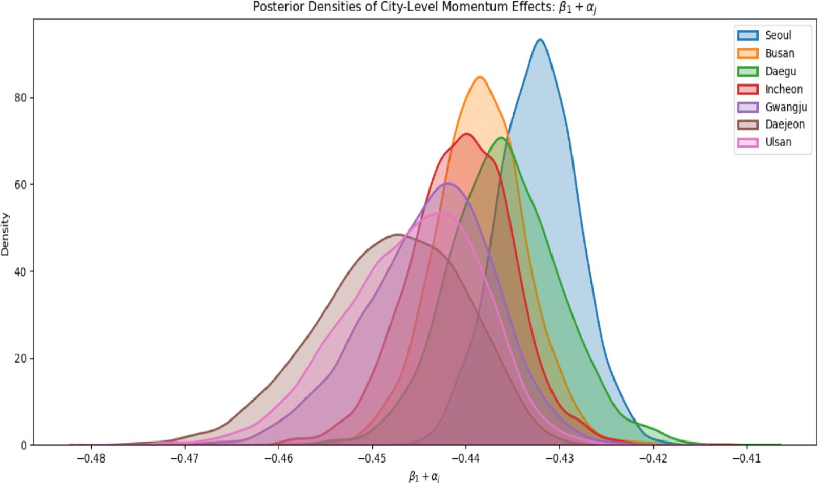
<Table 6> summarizes the posterior means and 90% HDIs for each city’s momentum coefficient. These values quantify the degree of responsiveness of current housing price changes to past changes, along with the associated uncertainty in each city-specific estimate.
Note: β1+αj measures the persistence of monthly housing price changes in each city. Higher positive values indicate momentum, while negative values imply mean reversion. All cities show negative values, consistent with the presence of corrective price dynamics. HDI refers to high density interval. Units are expressed in percentage points.
Building on the regional heterogeneity identified in the previous sections, we now assess whether spatial patterns are present in the distribution of housing price momentum effects by computing Moran’s I statistics at both the city and district levels. Moran’s I (i.e., Moran, 1950) is a widely used global indicator of spatial dependence, measuring whether areas with similar values of a variable—here, estimated momentum coefficients—tend to be geographically clustered or dispersed. A significantly positive Moran’s I suggests spatial clustering of similar momentum effects, potentially reflecting regional spillovers or shared local dynamics. Conversely, a significantly negative value implies spatial dispersion, which may be interpreted as local divergence or competitive substitution between neighboring regions (Burchfield et al., 2006; Glaeser et al., 2005; Han & Strange, 2015).
<Table 7> presents the Moran’s I estimates, the expected values under the null hypothesis of spatial randomness, and associated p-values derived from permutation tests. At the city level, the Moran’s I is estimated at –0.2718, which is more negative than the theoretical expectation of –0.1667under spatial randomness. However, the result is not statistically significant (p=0.439), indicating that momentum effects do not exhibit meaningful spatial autocorrelation across cities. This suggests that city-level variation in momentum effects is largely idiosyncratic and not spatially structured, potentially reflecting differences in local policy regimes, demographic compositions, or housing supply elasticity that are not spatially contiguous.
Note: Moran’s I measures spatial autocorrelation in estimated momentum effects. For the construction of spatial weights, the number of nearest neighbors was set to k=4 by default. In cases where the number of spatial units was limited (e.g., Ulsan, Daejeon, and Gwangju), the number of neighbors was set to k=3 to ensure a valid weight matrix.
At the district-level, spatial autocorrelation is generally weak across most metropolitan areas. Moran’s I values for Seoul, Incheon, Busan, Daejeon, Gwangju, and Ulsan are close to zero or moderately negative and statistically insignificant. These findings imply that, within these cities, district-level momentum effects do not demonstrate strong spatial clustering. Such results may be attributed to the relatively small number of spatial units (i.e., districts), limited spatial granularity of the effects, or heterogeneous intra-city housing dynamics that dilute broader spatial patterns.
An important exception is Daegu, where the Moran’s I is significantly negative at –0.2949 (p=0.018), revealing strong spatial heterogeneity. This implies that districts with above-average momentum effects are likely to be surrounded by districts with below-average effects, and vice versa. Such local divergence may reflect sharp differences in neighborhood-level fundamentals, such as redevelopment intensity, school quality, or localized investment behavior. The presence of spatial dispersion within Daegu underscores the importance of modeling intra-urban dynamics explicitly when designing policy interventions or forecasting price dynamics at sub-city scales.
V. Tests on Momentum Strategies in the Korean Housing Market
This study examines the momentum trading strategy described by Jegadeesh & Titman (1993) in the context of the South Korean housing market to assess its effectiveness. The strategy involves forming portfolios based on the historical performance of properties, buying those that have recently performed well (“winners”), and short-selling those that have underperformed (“losers”). A distinguishing aspect of this study is the consideration of real-world frictions such as capital gains taxes and transaction fees, which are significant in the housing market. By factoring in these elements, the study offers a more practical assessment of the strategy’s potential profitability.
The dataset used contains monthly transaction-level records for apartment properties in major cities across South Korea, including Seoul, Busan, Daegu, Incheon, Gwangju, Daejeon, and Ulsan. The data spans from January 2015 to December 2023. Unlike the continuous trading of stocks in equity markets, the housing market data forms an unbalanced panel due to irregular transaction frequencies. This means that some properties are bought and sold multiple times, while others are infrequently traded. This unbalanced nature presents a challenge for momentum strategy analysis, as it requires careful handling of gaps in transaction history.
To address this, we calculate the cumulative returns for each unit only using the months in which transactions are recorded. This helps to avoid biases that can be introduced by inactive periods. By concentrating on active transaction months, the study ensures that the momentum signals are based on genuine market activity rather than artificially smoothed data. This approach gives a more accurate measure of historical performance, reflecting the true trading opportunities available to investors.
The momentum strategy is implemented by forming portfolios at the end of each month based on the cumulative returns of properties over a formation period, Tf, and holding them for a specified holding period, Th. Both Tf and Th are varied to capture different market dynamics. The formation period (e.g., 3, 6, 9, or 12 months) is used to identify momentum signals, while the holding period (e.g., 3, 6, 9, or 12 months) allows us to test the persistence of these signals.
The cumulative return for property i over the formation period is calculated as:
Where ri,t is the monthly return of unit i in month t. This compounding captures the multiplicative effects of gains and losses over time, providing a robust measure of past performance.
At the end of each formation period, housing units are ranked based on their cumulative returns. The top-performing units (i.e., top 10 percentile) are grouped into a “winner” portfolio, while the bottom performers (i.e., bottom 10 percentile) constitute the “loser” portfolio. During the subsequent holding period, these portfolios are held, and their performance is tracked. This procedure is repeated monthly, generating a time series of returns for both winner and loser portfolios, which allows us to evaluate the strategy’s effectiveness across different market conditions.
An important expansion of this study compared to Jegadeesh & Titman (1993) is the consideration of taxes and transaction fees, both of which have a substantial impact on the profitability of real estate investments. In the Korean housing market, these costs are significant and can vary based on market conditions and the size of the transaction.
The South Korean government imposes a progressive tax on capital gains, based on the year of the transaction and the amount of the gain. We have implemented a detailed tax structure to determine the net return for investments in residential properties. The tax structure for housing properties is outlined in <Table 8>, demonstrating the progressive nature of the tax system.
For each transaction, the capital gain for property i is calculated as:
Where Pi,sell represents the sale price at the end of the holding period, and Pi,buy represents the purchase price at the beginning of the formation period. The tax structure is then used to apply the applicable tax rate and deduction in order to compute the tax amount.
This tax calculation ensures that the simulated net returns reflect the actual costs investors would face, providing a realistic measure of post-tax performance. In addition to taxes, real estate transactions incur various fees, such as brokerage commissions and legal costs. We model these fees as a fixed percentage, δ = 0.5%, of the transaction price. The total transaction fee for property i is expressed as:
We conducted simulations using various combinations of formation (Tf) and holding periods (Th) to examine how the momentum effect is influenced by the investment horizon and reference point. The primary outcome of these simulations is the average net return, which signifies the effectiveness of the strategy after accounting for taxes and fees.
The heatmap in <Fig. 6> demonstrates the performance of momentum strategies in the housing market, considering various formation and holding periods. The results indicate that all tested combinations of formation and holding periods resulted in negative returns. Notably, strategies with short formation and holding periods exhibited the most significant negative returns. This suggests that when momentum strategies rely on a brief historical period for portfolio formation and execute trades over a short duration, transaction costs, and taxes significantly erode potential gains. The high turnover inherent in these short-term strategies amplifies the impact of fees and taxes, leading to a rapid decline in net returns.
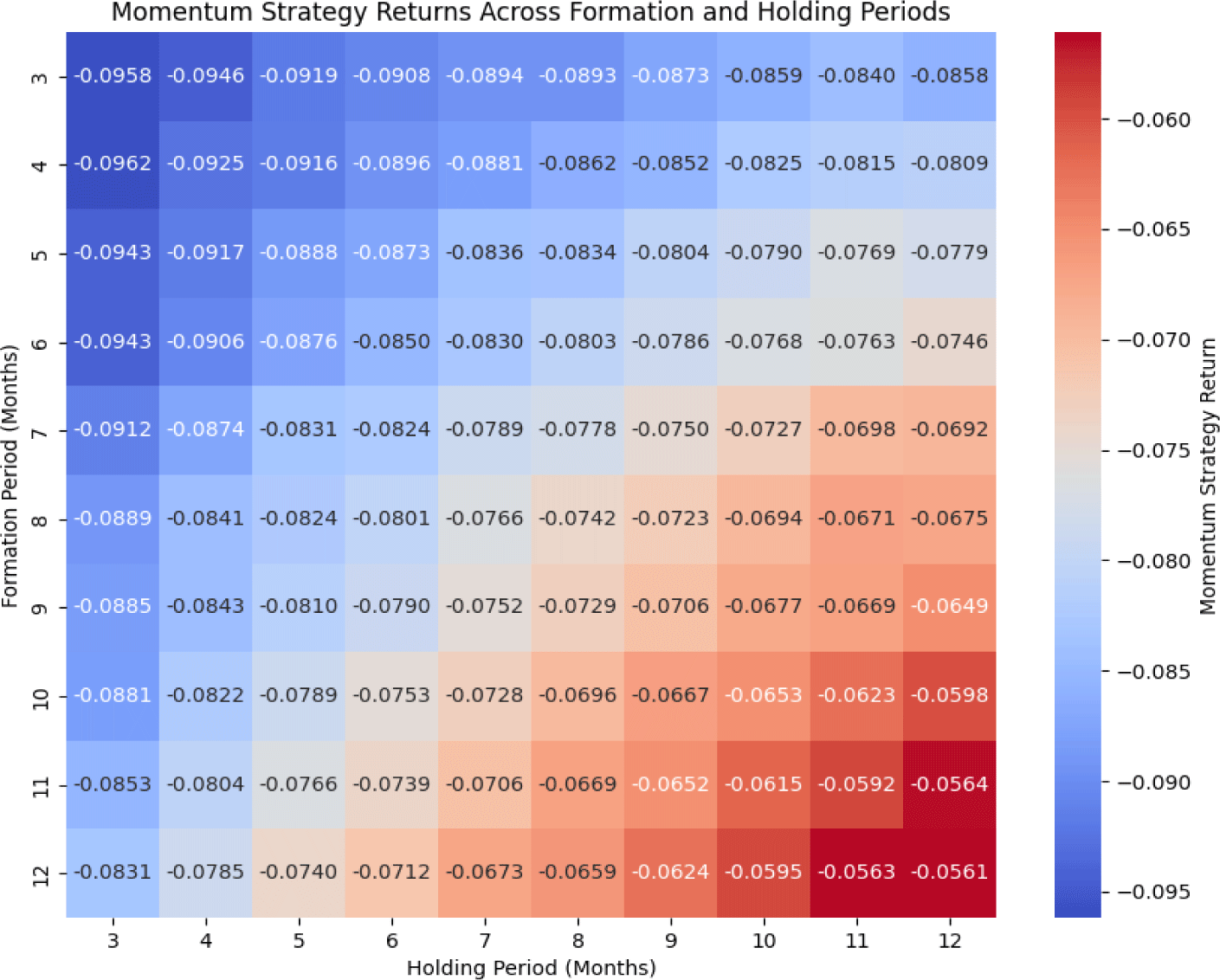
This pattern contrasts with findings from more liquid markets, such as equities, where momentum strategies often capitalize on short-term price trends (Asness et al., 2013; Jegadeesh & Titman, 1993). The negative results in the housing market underscore the unique challenges posed by real estate investments, including lower liquidity, higher transaction costs, and the relatively slow adjustment of prices. These market-specific factors impede the success of momentum strategies, especially when high-frequency trading is involved.
Interestingly, as both the formation and holding periods extend, the magnitude of negative returns diminishes, although they remain negative overall. This trend indicates that longer formation periods may allow for a more accurate capture of underlying price momentum in the housing market, and extended holding periods help mitigate the adverse effects of repeated transaction costs. However, even with these adjustments, the momentum strategy does not produce positive returns when taxes and fees are factored in.
In summary, the analysis suggests that using traditional momentum strategies in the Korean housing market is significantly limited by the market’s structural characteristics. The consistent negative returns, especially in short-term strategies, emphasize the need for investors to reconsider using momentum-based approaches in real estate.
In this section, we are examining the performance of momentum strategies while considering the constraint that short sales are not allowed. This adjustment reflects a more realistic scenario for many housing markets, including South Korea, where short-selling properties are either legally restricted or practically infeasible due to high transaction costs, market regulations, and the illiquid nature of real estate assets. By excluding short positions from our strategy, we aim to assess the effectiveness of momentum trading when investors are limited to long-only positions.
In the traditional momentum strategy, both “winners” (top-performing assets) and “losers” (bottom-performing assets) are included in the portfolio, with investors taking long positions in the winners and short positions in the losers. To modify this strategy for a long-only framework, we adjust the portfolio construction as follows:
-
- At the end of each formation period, properties are ranked based on their cumulative returns. The properties in the top quantile (e.g., top 10%) are selected as “winners,” and the investor takes long positions in these properties.
-
- Instead of shorting the “losers,” the strategy simply avoids taking any position in the bottom-ranked properties. This means the portfolio is composed solely of long positions in the winner properties, eliminating the potential profits (or losses) from short positions.
This adjustment creates a momentum strategy that focuses on purchasing properties with a strong historical performance. Instead of potential short positions, the strategy involves holding cash or risk-free assets. However, because short-selling is not an option, the strategy’s ability to hedge against market downturns is limited, which affects the risk-return profile of the portfolio.
The performance of the long-only momentum strategy is evaluated across different combinations of formation and holding periods, similar to the standard momentum strategy. The heatmap in <Fig. 7> illustrates the performance of the momentum strategy when short-selling is not permitted.
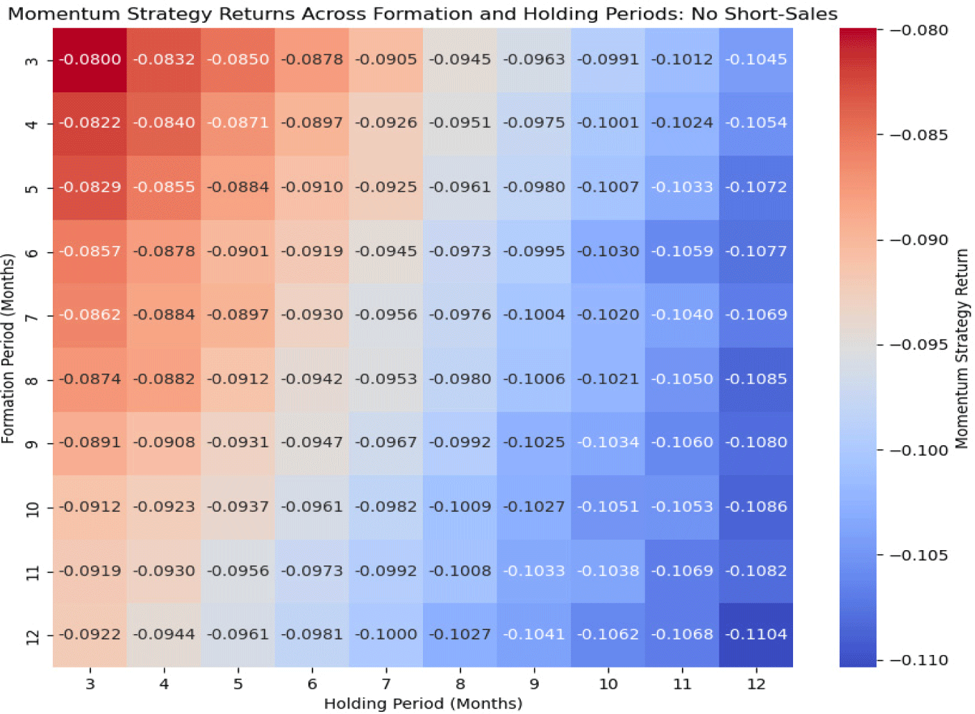
One important difference in this heatmap is the generally more negative returns seen across almost all combinations of formation and holding periods compared to the earlier results. Returns become increasingly negative as both the formation and holding periods get longer. For instance, the returns for longer formation periods (9 to 12 months) and holding periods (8 to 12 months) drop below –0.10, indicating a more significant decrease in returns in these cases. This suggests that when short-selling is restricted, extending the formation and holding periods leads to progressively worse performance of the momentum strategy in the housing market.
The exclusion of short-selling in the previous heatmap resulted in more noticeable negative outcomes compared to when both long and short positions were considered. The earlier results showed less severe negative returns, especially for shorter formation and holding periods. This suggests that including short positions may have helped counter some of the adverse effects. Without the ability to short-sell, the strategy lacks flexibility to hedge against potential market downturns, leading to more pronounced underperformance.
Additionally, the heatmap shows that even with shorter formation periods (3 to 5 months) and shorter holding periods, the returns are still negative, though not as steep as with longer-term strategies. This suggests that simply holding onto winning investments without the ability to sell losing investments short does not lead to positive returns in the housing market. The adverse effects of transaction fees and taxes are more noticeable in this long-only strategy, emphasizing that these costs have a significant impact on net returns.
The analysis results offer important insights into the difficulties of using momentum strategies in the Korean housing market. This is especially true when taking into account market frictions like taxes, transaction fees, and the inability to short-sell. Regardless of the different formation and holding periods, the momentum strategy mostly results in negative returns. This suggests that the dynamics of the housing market are quite different from more liquid markets such as equities, where momentum strategies have historically been more effective.
To further explore the policy relevance of these findings, we extend the analysis by evaluating the effect of a tax increase on momentum-based investment returns in the following subsection.
To investigate how housing-related tax policy affects investment returns, we simulate the momentum strategy under a 25 basis point (bps) increase in the capital gains tax schedule. The simulation assumes a long-only portfolio without short-sales and includes realistic transaction. <Fig. 8> reports the average returns across various formation and holding period combinations.
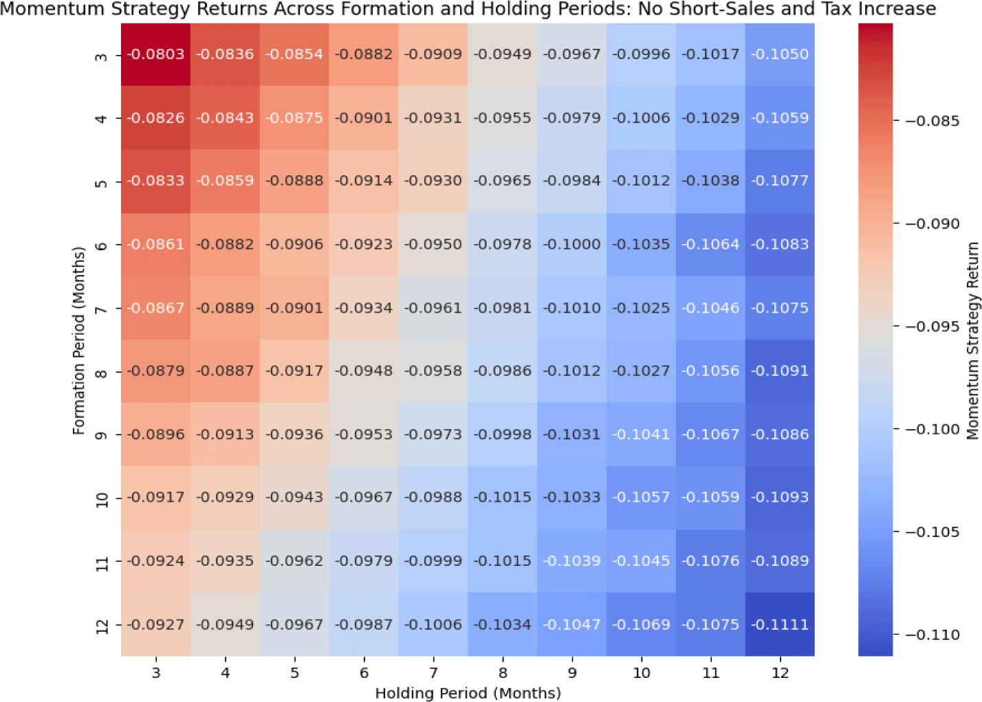
Compared to the baseline case without a tax increase (<Fig. 7>), the introduction of a higher tax burden leads to a consistent decline in post-tax momentum returns across all parameter configurations. The magnitude of this decline increases with the holding period, reflecting the cumulative impact of taxation over time. For example, when using a 12-month formation period and a 12-month holding period, the average return decreases from –0.1104 in the baseline case to –0.1111 under the tax hike scenario. Although numerically modest, this reduction accumulates over time and can significantly alter the profitability of housing investment strategies.
These results highlight the importance of incorporating policy-induced frictions into the evaluation of asset return dynamics. Tax increases, even if moderate, erode momentum-based profits and can partially offset behavioral pricing anomalies in the housing market. We note that further extensions—such as differentiated tax treatments by holding period—could yield richer implications and are left for future work.
VI. Conclusion and Policy Implications
This study provides a comprehensive analysis of momentum effects in South Korea’s housing market using monthly transaction-level data and a Bayesian hierarchical framework. By accounting for both city- and district-level heterogeneity, the study highlights how momentum patterns differ across regions and how these patterns interact with factors such as market liquidity, price volatility. The results have important implications for housing market policy and investment strategy.
From a policy perspective, our findings underscore the need for regionally differentiated interventions. Although the national average suggests a mean-reverting tendency in price dynamics, cities such as Seoul exhibit relatively strong momentum effects that partially offset this trend. These localized deviations suggest that blanket policy measures may be insufficient or even counterproductive. Instead, more targeted approaches—such as differential loan-to-value (LTV) or debt-to-income caps, tailored tax incentives, or localized housing supply initiatives—could more effectively address region-specific market pressures. For example, districts with strong upward momentum and limited supply could benefit from regulatory measures to expand housing availability or dampen speculative demand. Conversely, regions with weaker or mean-reverting dynamics may require less aggressive intervention.
Our simulation results provide additional policy insight by demonstrating that momentum-based investment strategies yield negative or near-zero net returns once real-world frictions, such as transaction fees and capital gains taxes, are considered. This finding suggests that existing tax structures and market frictions already serve as effective constraints on speculative trading behavior. Therefore, in regions where momentum is still observed despite these frictions—such as parts of Seoul—policymakers may need to consider complementary tools such as targeted supply-side measures or more aggressive taxation to curb excessive price persistence.
Moreover, the ineffectiveness of momentum strategies under short-sales constraints highlights the structural limitations of Korea’s housing market in facilitating arbitrage and timely price correction. This suggests that in the absence of mechanisms to offset overvaluation—such as short-selling or more dynamic trading instruments—policy interventions may play a more critical role in mitigating excessive price persistence and ensuring market stability.
Despite its contributions, this study has several limitations that offer avenues for future research. First, our definition of homogeneous housing units relies on observable characteristics—such as apartment name, exclusive area, and construction year—due to the absence of unique unit identifiers in publicly available data. This approach may introduce measurement error that could attenuate estimates of momentum or mean-reverting effects. Future work could address this limitation by leveraging administrative or proprietary datasets with finer unit-level resolution.
Second, although we examine spatial autocorrelation ex post using Moran’s I, we do not incorporate spatial priors such as conditional autoregressive (CAR) or intrinsic CAR structures into the model due to computational constraints. Extending the hierarchical Bayesian framework to include spatially structured priors would allow for a more rigorous estimation of spatial spillovers in housing price dynamics.
Third, while we conduct a simulation to evaluate the impact of a capital gains tax increase, our analysis does not fully examine the broader array of policy instruments—such as differentiated capital gains tax schedules based on holding periods, property tax reforms, region-specific LTV caps, or targeted housing supply interventions—that could more comprehensively inform strategies for stabilizing the housing market. Expanding the policy simulation framework to include these levers represents a promising direction for applied policy research.
Fourth, although we document substantial spatial heterogeneity in momentum effects across cities and districts, we do not empirically identify the structural drivers behind these variations. A deeper examination of factors such as institutional constraints, infrastructure access, demographic composition, or speculative activity would enhance our understanding of regional dynamics and improve the generalizability of policy recommendations.
Finally, in constructing the monthly panel dataset, we adopt a within-month LOCF rule to define end-of-month housing prices. While this approach reduces spurious temporal correlations, it also necessitates the exclusion of units with sparse trading histories, potentially biasing the sample toward more liquid units. Future research could explore imputation-based or model-based approaches to more flexibly address sparsity in transaction timing, thereby improving the representativeness of the analysis.
Taken together, these findings contribute to a more granular understanding of housing price dynamics in a non-Western context and provide a foundation for future research on spatially targeted housing policy design.